
Control is why we care
Prediction is not the point. Control is.


In the previous blogs, we built the foundations of world models:
What a world model is
Why partial observability forces us to maintain a belief state
How linear (Kalman filtering) and nonlinear approximations maintain that belief
At this point, we could take a detour. We could ask a different question:
Instead of asking “What is the belief over the hidden state?”,
we could ask “What internal variables minimize prediction error?”
That would lead us to predictive coding and variational free energy: a shift in perspective from state estimation to error minimization.
But we are not going there yet. Because we are still missing something more fundamental: Why do we build models at all?
A belief state is not the end goal. Control is.
Before we move into deep neural world models, we must understand classical model-based control. Only then will it be clear what modern world models are approximating.
Why Models Exist
A model is not built for reconstruction. A model is built for counterfactual reasoning. If I take action a, what happens next?
Without a model, control becomes reactive. With a model, control becomes anticipatory.
The entire motivation for world models is this shift: From reacting to observations to reasoning about imagined futures.
Classical control theory already solved this problem, but under strong assumptions. Modern world models relax those assumptions. But the structure is the same.
When Control Becomes Planning
Before getting into neural world models, we need to understand something much simpler: What happens when we know the dynamics?
Let’s start with the most classical case.
Linear Quadratic Regulator (LQR)
We assume linear dynamics:
And a quadratic cost:
where:
Q >= 0 penalizes state deviation
R > 0 penalizes control effort
And we get the optimal policy to be linear:
where K comes from solving the Riccati Equation.
I think this is stunning:
The value function is quadratic:
\(V(x) = x^TPx\)The optimal action is linear in state.
The entire problem has a closed-form global solution.
The control law is smooth and stable everywhere.
If I want to think about this geometrically, LQR works because the dynamics are linear, the cost is convex quadratic, and the value function remains quadratic under Bellman backup.
The system becomes a smooth energy landscape. Control is just pushing the system downhill — this is optimal control exploiting structure.
But what if we don’t want a fixed policy?
LQR gives us a static feedback law.
But suppose the system is nonlinear, there are constraints, the horizon is finite, and we care about the trajectory-level behavior. Instead of learning a policy, we can plan directly. This is Model Predictive Control.
Model Predictive Control (MPC)
Assume we know the dynamics:
At time t, we:
Observe the current state s_t.
Optimize a sequence of actions to maximize predicted reward over horizon H:
\(a_{t:t+H}^* = \text{argmax}_{a_{t:t+H}}\sum^H_{k=0} \gamma^k r (s_{t+k},a_{t+k})\)
subject to constraint:
Now, the crucial trick here is that we only execute the first action:
Then at the next step:
Observe the new state x_{t+1}
Re-solve the optimization
Re-plan
This is called Receding Horizon Control.
It is robust because model errors get corrected every step, the disturbances are absorbed via replanning, no fixed policy is required, and constraints can be handled naturally.
It trades analytic elegance for computational flexibility.
LQR solves the Bellman equation analytically.
MPC solves the Bellman numerically at every step.
It performs trajectory optimization under dynamics constraints.
We’re gonna do a little experiment
First, we will learn a linear dynamics model from data (random actions in a 1D nonlinear system), then use random-shooting MPC to choose actions: sample many action sequences, roll them out with the learned model, and pick the one with the lowest predicted cost (quadratic in state and action)
import numpy as np
import matplotlib.pyplot as plt

np.random.seed(0)

# TRUE environment (unknown dynamics)
def f_true(x, a, noise_std=0.02):
    return 0.9*x + 0.2*np.sin(x) + a + noise_std*np.random.randn()

# -----------------------------
# Learned model class: linear regression
# x_{t+1} ≈ theta0 + theta_x * x_t + theta_a * a_t
# -----------------------------
def fit_linear_dynamics(xs, a_s, xnexts):
    # Design matrix: [1, x, a]
    X = np.stack([np.ones_like(xs), xs, a_s], axis=1)  # shape (N,3)
    y = xnexts.reshape(-1, 1)                          # shape (N,1)
    # theta = (X^T X)^{-1} X^T y  (least squares)
    theta, *_ = np.linalg.lstsq(X, y, rcond=None)
    return theta.flatten()  # [theta0, theta_x, theta_a]

def f_hat(theta, x, a):
    return theta[0] + theta[1]*x + theta[2]*a

# MPC via random shooting
def mpc_action(theta, x0, H=15, K=2000, a_max=1.0, q=1.0, r=0.05):
    """
    Sample K candidate action sequences length H, simulate under learned model,
    choose lowest predicted cost. Return first action.
    """
    best_cost = float("inf")
    best_a0 = 0.0

    # Sample actions uniformly in [-a_max, a_max]
    A = np.random.uniform(-a_max, a_max, size=(K, H))

    for k in range(K):
        x = x0
        cost = 0.0
        for t in range(H):
            a = A[k, t]
            cost += q*(x*x) + r*(a*a)
            x = f_hat(theta, x, a)
        if cost < best_cost:
            best_cost = cost
            best_a0 = A[k, 0]

    return best_a0, best_cost

# 1) DATA COLLECTION (random actions)
def collect_data(N=2000, a_max=1.0):
    xs = []
    a_s = []
    xnexts = []
    x = 1.5  # start away from zero

    for _ in range(N):
        a = np.random.uniform(-a_max, a_max)
        x_next = f_true(x, a)
        xs.append(x)
        a_s.append(a)
        xnexts.append(x_next)
        x = x_next
    return np.array(xs), np.array(a_s), np.array(xnexts)

xs, a_s, xnexts = collect_data(N=2500, a_max=0.6)

theta = fit_linear_dynamics(xs, a_s, xnexts)
print("Learned theta [bias, x_coeff, a_coeff] =", theta)

# 2) CONTROL with MPC (learned model)
T = 80
H = 18
K = 2500

# Mismatch knob: during control, we can change the true system slightly
def f_true_mismatched(x, a, noise_std=0.02):
    # stronger nonlinearity + slight gain shift (distribution shift)
    return 0.85*x + 0.35*np.sin(1.2*x) + a + noise_std*np.random.randn()

x = 2.2  # initial state for control
traj = [x]
acts = []
pred_costs = []

for t in range(T):
    a, predJ = mpc_action(theta, x, H=H, K=K, a_max=1.0, q=1.0, r=0.05)
    # execute in the REAL environment (mismatched)
    x = f_true_mismatched(x, a)
    traj.append(x)
    acts.append(a)
    pred_costs.append(predJ)

traj = np.array(traj)

# 3) Compare against "oracle MPC" that uses the TRUE model (for reference)
def mpc_action_oracle(x0, H=15, K=2000, a_max=1.0, q=1.0, r=0.05):
    best_cost = float("inf")
    best_a0 = 0.0
    A = np.random.uniform(-a_max, a_max, size=(K, H))
    for k in range(K):
        x = x0
        cost = 0.0
        for t in range(H):
            a = A[k, t]
            cost += q*(x*x) + r*(a*a)
            x = f_true_mismatched(x, a, noise_std=0.0)  # deterministic planning
        if cost < best_cost:
            best_cost = cost
            best_a0 = A[k, 0]
    return best_a0

x2 = 2.2
traj_oracle = [x2]
acts_oracle = []
for t in range(T):
    a2 = mpc_action_oracle(x2, H=H, K=K, a_max=1.0, q=1.0, r=0.05)
    x2 = f_true_mismatched(x2, a2)
    traj_oracle.append(x2)
    acts_oracle.append(a2)

traj_oracle = np.array(traj_oracle)
Here, MPC with a learned model is compared to an oracle that uses the true dynamics. During control, the true system is changed (stronger non-linearity, different gain), so the learned model is wrong.
The plots show that MPC with the learned model fails to regulate the state to zero and can diverge, while oracle MPC succeeds.
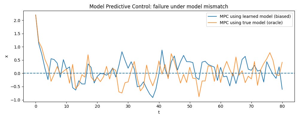

The takeaway is that model error breaks MPC; the controller trusts its model and plans with it, so when the model is wrong, the resulting actions can be poor or destabilizing — what we know as model bias.
Now the important bridge
Modern neural world models do something strikingly similar. They
Maintain a belief state (like Kalman filtering)
Roll out imagined trajectories
Evaluate candidate futures
Pick the best first action
Re-plan the next timestep
This is nothing but approximate MPC in latent space.
The only thing that changes is:
And
Classical control solves trajectory inference in physical state space. Neural world models solve trajectory inference in learned latent space.
Modern neural world models can be viewed as nonlinear belief filters coupled with approximate model predictive control in latent space.
Please note that even if Kalman filters and MPC are optimal, we need Neural World Models because of the dimensionality curse (pixel dimensions, inverting the matrix in Kalman Gain is O(D^3), non-linearity (real-world dynamics are rarely linear), and unknown state spaces (till now, we worked with state (position, velocity), we will deal with pixels, we need to learn what the state is).
What breaks with high-dimensional observations (pixels)?
We know that classical assumptions require:
known observation model
low-dimensional x_t
tractable likelihood
Pixels violate all three
observation noise is structured, not Gaussian
likelihood is unknown
observations:
\(o_t \in R^{H \times W \times C}\)
What are the consequences?
Filtering is impossible without representation learning.
Particle filters collapse instantly or “PF dies.”
EKF linearization is meaningless or “EKF lies.”
State is no longer “given”, it must be learned
This is the exact point where neural world models become inevitable.
A few research questions to consider at the end
Can we get identifiable latent states without strong inductive biases?
When is uncertainty actually needed for control?
Can belief compression be task-adaptive?
Is filtering the right abstraction for learning agents, or just a convenient one?
What’s next?
Finally, in the next blog, I’m going to introduce neural world models - talk about high-dimensional observations, what happens if we try to just predict pixels directly, and how we can fix that by introducing a latent state.
~Ashutosh