
Filtering is the original world model
A world model is a belief updater + predictor


We’re going to derive the latent state and belief state view that we discussed in the last blog. Assume the environment has an unobserved “true” state x_t evolving with controlled dynamics:
We don’t observe x_t. We observe o_t, which may be aliased (many x map to similar o). From the agent’s perspective, the only rational internal object is a distribution over possible current states given history:
Now, we will derive the belief state using Bayes filtering and marginalization updates.
Before Recurrent Neural Networks (RNNs), this was solved via Recursive Bayesian Estimation. We want the posterior belief of the current state given history.
This update consists of two steps, which we will see mirrored in every modern neural architecture (from Kalman Filters to Transformers). We will also see how prediction and correction are distinct operations:
Prediction Step (The “Prior” or “Imagination”): Before seeing observation x_t, we project our “belief” forward based on the previous state and action:
\(p(s_t|x_{1:t},a_{1:t-1}) = \int \underbrace{p(s_t|s_{t-1},a_{t-1})}_\text{Dynamics}\underbrace{p(s_{t-1}|x_{1:t-1},a_{1:t-2})}_\text{Previous Posterior}ds_{t-1}\)Update Step (The “Correction” or “Observation”): We incorporate the new observation x_t using Bayes’ rule:
\(p(s_t|x_{1:t},a_{1:t-1}) \propto \underbrace{p(x_t|s_t)}_\text{decoder}\underbrace{p(s_t|x_{1:t-1},a_{1:t-1})}_\text{Prediction(Prior)}\)
One research insight here is that modern architectures like Dreamer or RSSM are just variational approximations of these two integrals.
The RNN hidden state usually carries the Prediction
The VAE Encoder performs the Update
The “world model” in the partially observed case is fundamentally learning (or approximating) two coupled things:
a dynamics model in some state space
an inference/decode/update rule that maps history to state (belief)
In modern neural world models, we typically replace the belief state by a parameteric latent z_t meant to approximate either a point estimate of belief or a distributional belief.
What do we mean by Bayesian Filtering?
Filtering is exactly the belief recursion derived above (predict and update). World models are essentially: learn a filter + a predictive transition in a representation that’s tractable.
In the last blog, we mentioned:

The Markov assumption is not “the environment is memoryless”. Instead, there exists a state x_t such that:
In such Partially Observable Markov Decision Processes (POMDPs), the observation o_t is generally NOT Markov.
A raw frame stack is a crude approximation. A learned latent is a better one if trained correctly.
Belief is Markov, but expensive.
The belief b_t is infinite-dimensional in continuous spaces. Here are a few practical approximations that we use:
Gaussian belief (Kalman filter-style)
Particle belief (Particle filter (PF)-style)
Learned latent belief (Neural encoder + Recurrence)
It’s totally all right to address a key design choice now: Do we represent uncertainty explicitly (distribution over state), or do we compress to a point state and hope the policy absorbs uncertainty?
This trade-off will reappear as stochastic vs deterministic latents later.
Can we derive the Kalman filter using the belief recursion?
We saw earlier that the belief state can be approximated as Gaussian (Kalman filter-style, linear here). With approximations come assumptions (strong here)
Before anything, if you observe the belief state as a Gaussian approximation, we have “covariance”, and keep wondering if it can be used as an “uncertainty” budget. We’ll address this later.
Anyways, the assumption here is that the belief remains Gaussian forever.
Let’s get into the derivation. Don’t get intimidated by the characters; it’s very simple.
Prediction step
We know that Gaussian + affine map => Gaussian:
Correction step: Multiply the prior by the likelihood
Product of Gaussian => Gaussian with:
This is the Kalman filter, but please note that it’s nothing more than exact Bayesian filtering under the linear-Gaussian assumption.
Why does this matter for world models?
The above gives us:
a belief state (mean, variance)
a deterministic prediction step
a data-dependent correction step
Every modern neural world model recreates this structure:
deterministic transition
stochastic belief
encoder acting as corrector
At last, here’s a code implementation of a 1D (linear, what we derived above) Kalman filter:
import math, random
import matplotlib.pyplot as plt

# 1D Kalman Filter from scratch
# x_{t+1} = x_t a_t + eps, eps ~N(0, Q)
# o_t = x_t + eta, eta ~N(0, R)

def randn():
    u1 = max(1e-12, random.random())
    u2 = random.random()
    z = math.sqrt(-2.0*math.log(u1))*math.cos(2.0*math.pi*u2)
    return z

def simulate(T=100, x0=0.0, Q=0.2**2, R=0.6**2):
    '''
    Simulate true states x_t and observations o_t, with controls a_t.
    Args:
        T: number of time steps
        x0: initial state
        Q: process noise variance
        R: observation noise variance
    Returns:
        x: true states
        o: observations
        a: controls
    '''

    x = [0.0]*(T+1)
    o = [0.0]*(T+1)
    a = [0.0]*(T+1)

    x[0] = x0
    o[0] = x[0] + math.sqrt(R)*randn()

    # Example control profile
    for t in range(T):
        a[t] = 0.2 * math.sin(2.0*math.pi*t/T) + 0.02
        x[t+1] = x[t] + a[t] + math.sqrt(Q)*randn()
        o[t+1] = x[t+1] + math.sqrt(R)*randn()

    return x, o, a

def kalman_filter_1d(o, a, mu0=0.0, sigma0=1.0, Q=0.2**2, R=0.6**2):
    '''
    Kalman filter for 1D linear dynamic system.
    Belief at time t: x_t ~ N(mu_t, sigma_t)
    Args:
        o: observations
        a: controls
        mu0: initial mean
        sigma0: initial variance
        Q: process noise variance
        R: observation noise variance
    Returns:
        mu: posterior mean
        P_sigma: posterior variance
    '''
    T = len(o) - 1
    mu = [0.0]*(T+1)
    P_sigma = [0.0]*(T+1)

    mu[0], P_sigma[0] = mu0, sigma0

    for t in range(T):
        # Prediction step
        mu_pred = mu[t] + a[t]
        P_pred = P_sigma[t] + Q

        # Update step, Correction using observation o_{t+1}
        y = o[t+1] - mu_pred # innovation
        S = P_pred + R # innovation covariance
        K = P_pred / S # kalman gain (scalar)

        mu[t+1] = mu_pred + K * y
        P_sigma[t+1] = (1 - K) * P_pred

    return mu, P_sigma

# Demo
random.seed(42)
T=120
Q = 0.15**2
R = 0.50**2

x_true, o, a = simulate(T, x0=-1.0, Q=Q, R=R)
mu,P_sigma = kalman_filter_1d(o, a, mu0=0.0, sigma0=1.5**2, Q=Q, R=R)

t = list(range(T+1))
sigma = [math.sqrt(max(0.0, P)) for P in P_sigma]
upper = [m + 2*s for m,s in zip(mu, sigma)]
lower = [m - 2*s for m,s in zip(mu, sigma)]

plt.figure(figsize=(10, 6))
plt.plot(t, x_true, label="true $x_t$")
plt.plot(t, mu, label="belief mean $\\mu_t$")
plt.fill_between(t, lower, upper, alpha=0.2, label="$\\mu_t \\pm 2\\sigma_t$")
plt.scatter(t, o, s=10, alpha=0.25, label="observations $o_t$")
plt.xlabel("t")
plt.ylabel("state / observation")
plt.title("1D Kalman Filter: random-walk + control, noisy observations")
plt.legend(loc="best")
plt.tight_layout()
plt.show()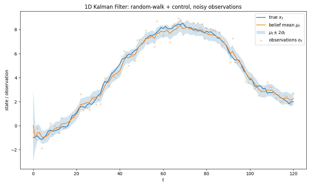
What’s next?
In this blog, we explored the linear approximation of the belief state. In the next post, we will discuss non-linearity and multimodality, and discover why the Extended Kalman Filter (EKF) lies, and the Particle Filter (PF) dies.
~Ashutosh