
Nonlinearity + Multimodality: why EKF lies and PF dies?
Approximate inference isn't optional, it's inevitable.


In the previous blog, we derived the belief or latent view under linear-Gaussian assumptions.
Now, we will relax just one assumption and operate under non-linearity:
Belief recursion is unchanged, and tractability is destroyed. Introducing the Extended Kalman Filter (EKF), in which the nonlinearity will be locally linearized. Let’s see how:
Approximate f,g via first-order Taylor expansion around the mean:
Then, we’re gonna pretend it’s linear Gaussian and reuse Kalman equations. One hidden (or much clearer in fact) assumption here is that the uncertainty is small and locally linear.
By doing this, what are the failure modes?
highly nonlinear dynamics
multimodal beliefs
contacts between agents, discontinuities
This will later appear as posterior collapse and overconfident latents in neural world models.
Now, it’s time to introduce another approximator - Particle Filter (PF). In one line, it can be stated as “sampling instead of parametrics”. You remember belief state derivation (check here), right? We’re gonna represent belief as (please note that the belief was unchanged in EKF):
Now, the belief state has changed, we’ll need to change the “Prediction” and “Correction” step as well (belief recursion update has changed with the definition of belief state).
And then, we resample again.
From sampling, what do we gain?
arbitrary nonlinearity
multimodal belief
What did we lose?
curse of dimensionality
sample degeneracy (I’m gonna explain this in a bit)
In fact, this is exactly why we later compress the belief state into low-dimensional learned latents to avoid sample inefficiency.
Why does EKF fail?
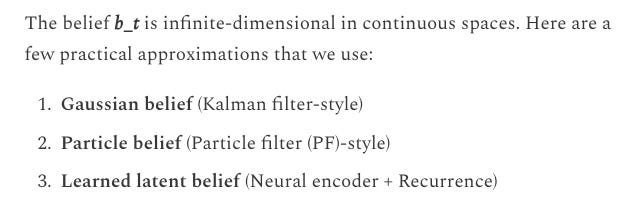
Let’s write a clean script to analyze EKF vs PF:
import math, random
import matplotlib.pyplot as plt

# Nonlinear System
# x_{t+1} = sin(x_t) + a_t _ eps, eps ~ N(0, Q)
# o_t = x_t^2 + eta, eta ~ N(0, R)

def randn():
    u1 = max(1e-12, random.random())
    u2 = random.random()
    z = math.sqrt(-2.0*math.log(u1))*math.cos(2.0*math.pi*u2)
    return z

def normal_pdf(x, mean, variance):
    if variance <= 0.0:
        return 0.0
    return (1.0 / math.sqrt(2.0+math.pi*variance)) * math.exp(-0.5*(x-mean)**2/variance)

def simulate_nonlinear_system(T=120, x0 = 0.7, Q=0.12**2, R=0.25**2):
    x = [0.0]*(T+1)
    o = [0.0]*(T+1)
    a = [0.0]*(T+1)

    x[0] = x0
    o[0] = x[0]**2 + math.sqrt(R)*randn()

    for t in range(T):
        a[t] = 0.2 * math.sin(2.0*math.pi*t/T) - 0.02
        x[t+1] = math.sin(x[t]) + a[t] + math.sqrt(Q)*randn()
        o[t+1] = x[t+1]**2 + math.sqrt(R)*randn()

    return x, o, a

def ekf_1d(o, a, mu0=0.0, sigma0=1.0, Q=0.12**2, R=0.25**2):
    '''
    Extended Kalman filter for 1D nonlinear dynamic system.
    Belief at time t: x_t ~ N(mu_t, sigma_t)
    Args:
        o: observations
        a: controls
        mu0: initial mean
        sigma0: initial variance
        Q: process noise variance
        R: observation noise variance
    '''
    T = len(o) - 1
    mu = [0.0]*(T+1)
    P_sigma = [0.0]*(T+1)

    mu[0], P_sigma[0] = mu0, sigma0

    for t in range(T):
        # Prediction step
        mu_pred = math.sin(mu[t]) + a[t]
        F = math.cos(mu[t])       # df/dx at mu[t]
        P_pred = F * P_sigma[t] * F + Q

        # Update with o_{t+1}
        H = 2.0 * mu_pred      # dh/dx at mu_pred
        z_pred = mu_pred * mu_pred
        y = o[t+1] - z_pred

        S = H * P_pred * H + R
        if S < 1e-12:
            mu[t+1], P_sigma[t+1] = mu_pred, max(P_pred, 1e-12)
            continue

        K = (P_pred * H) / S
        mu[t+1] = mu_pred + K * y
        P_sigma[t+1] = (1 - K * H) * P_pred
        P_sigma[t+1] = max(P_sigma[t+1], 1e-12)

    return mu, P_sigma

# Particle Filter for 1D nonlinear dynamic system.

def systematic_resample(particles, weights):
    N = len(particles)
    positions = [(random.random() + i) / N for i in range(N)]

    cumsum = []
    s = 0.0

    for w in weights:
        s += w
        cumsum.append(s)

    new_particles = [0.0]*N
    i=0
    for j, pos in enumerate(positions):
        while pos > cumsum[i]:
            i += 1
            if i >= N:
                i = N-1
                break
        new_particles[j] = particles[i]
    return new_particles

def particle_filter_1d(o, a, N=2000, x0_mean = 0.0, x0_std=1.0, Q=0.12**2, R=0.25**2, resample_threshold=0.5, seed=42):
    '''
    Particle filter for 1D nonlinear dynamic system.
    Belief at time t: x_t ~ sum_i w_i * delta(x_t - x_i)
    Args:
        o: observations
        a: controls
        N: number of particles
        x0_mean: initial mean
        x0_std: initial standard deviation
        Q: process noise variance
        R: observation noise variance
        resample_threshold: resample threshold
        seed: random seed
    Returns:
        mu: posterior mean
        P_sigma: posterior variance
        particles: particles
        weights: weights
    '''
    random.seed(seed)
    T = len(o) - 1
    particles = [x0_mean + x0_std*randn() for _ in range(N)]
    weights = [1.0/N]*(N)

    mean = [0.0]*(T+1)
    std = [0.0]*(T+1)

    def moments(ps, ws):
        m = sum(p*w for p,w in zip(ps, ws))
        v = sum(((p-m)**2)*w for p,w in zip(ps, ws))
        return m, math.sqrt(max(0.0, v))

    # weight using o_0
    for i in range(N):
        weights[i] *= normal_pdf(o[0], particles[i]**2, R)

    s = sum(weights)
    weights = [w/s for w in weights] if s != 0.0 else [1.0/N]*(N)
    mean[0], std[0] = moments(particles, weights)

    for t in range(T):
        # Propagate particles
        for i in range(N):
            particles[i] = math.sin(particles[i]) + a[t] + math.sqrt(Q)*randn()
        # Re-weight using 0_{t+1}
        for i in range(N):
            weights[i] = normal_pdf(o[t+1], particles[i]**2, R)

        s = sum(weights)
        weights = [w/s for w in weights] if s != 0.0 else [1.0/N]*(N)
        mean[t+1], std[t+1] = moments(particles, weights)

        # Resample if necessary or degeneracy
        ess = 1.0 / sum(w**2 for w in weights)
        if ess < resample_threshold * N:
            particles = systematic_resample(particles, weights)
            weights = [1.0/N]*(N)

        mean[t+1], std[t+1] = moments(particles, weights)

    return mean, std, particles, weights

def rmse(x, x_hat):
    return math.sqrt(sum((a-b)**2 for a,b in zip(x, x_hat))/len(x))

# Run an experiment
random.seed(42)

T = 140
Q = 0.12**2
R = 0.25**2

x_true, o, a = simulate_nonlinear_system(T=T, x0=0.9, Q=Q, R=R)

mu_ekf, P_ekf = ekf_1d(o, a, mu0=0.0, sigma0=1.2**2, Q=Q, R=R)
sig_ekf = [math.sqrt(p) for p in P_ekf]

mu_pf, sig_pf, particles, weights = particle_filter_1d(o, a, N=2500, x0_mean=0.0, x0_std=1.2, Q=Q, R=R)

rmse_ekf = rmse(x_true, mu_ekf)
rmse_pf  = rmse(x_true, mu_pf)

print("Accuracy (lower is better):")
print(f"  EKF RMSE: {rmse_ekf:.4f}")
print(f"  PF  RMSE: {rmse_pf:.4f}")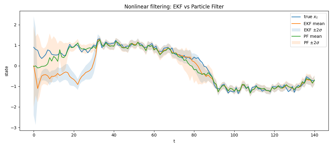
Based on these plots, we will try to answer a few questions.
1. What assumption did EKF silently violate?
The EKF didn’t fail because of “too much nonlinearity”. Instead, the violated assumption: EKF assumed the posterior is (approximately) Gaussian. More precisely:
and (local) linearization is used only to propagate the mean and covariance of that Gaussian.
The filter is therefore not estimating the true posterior, instead it’s estimating the best Gaussian approximation to the posterior.
For instance, based on our script and the plots:
In this case, the likelihood is symmetric:
Therefore, the posterior belief is bimodal:
Conclusively, we can say that two valid states explain the data equally well: x_t, -x_t.
This is NOT a Gaussian; this is a mixture distribution. What EKF does instead is compress the posterior into a single Gaussian. It places the belief at the mean of the modes. But the mean corresponds to a state that is actually unlikely!
So, the EKF is confidently wrong. The silent violation? The EKF requires: The posterior after nonlinear update remains approximately unimodal Gaussian.
2. Why does PF work?
The PF represents:
So, it naturally holds both near +x and -x. No Gaussian compression → no information loss.
EKF fails not when the dynamics are nonlinear. It fails when the posterior is not in the exponential family it represents.
This is the same failure mode as:
Gaussian latent variable models vs discrete latent reality
VAEs with unimodal latents vs multimodal futures
Diffusion vs deterministic predictors
Belief collapse in model-based RL
EKF silently assumed the belief remained Gaussian, but the measurement function created a multimodal posterior (state aliasing), violating identifiability.
Why does PF die?
It approximates the posterior:
using weighted samples (particles):
“PF dies” refers to the sample/particle degeneracy we mentioned earlier. It means:
Almost all particles get zero weight
Only 1-2 particles survive
The effective sample size collapses
Posterior approximation becomes useless
The weight update in PF:
Now, IF the likelihood is sharp, OR state dimension is large, OR proposal distribution is poor, OR model is highly nonlinear, OR the measurement noise is small, THEN most particles land in low-likelihood regions → their weights become ~0 → a few particles dominate.
The real problem is: Variance of importance weights grows exponentially wth dimension. In high dimensions:
The probability that a particle lands in a good region is tiny
We need exponentially many particles.
If the state dimension is d, then the required particles are approximately O(e^d).
So, PF “dies” because with practical particle counts, it cannot represent the posterior anymore.
What’s next?
In this blog, we discussed the nonlinear and multimodal estimation of the belief state using two approximators: EKF and PF, and discussed their lying and dying nature, respectively. Next, I would move on and discuss how much we care about “control” - how it moves from Linear Quadratic Regulator → Model Predictive Control → Model Bias. It’ll be a short blog.
~Ashutosh