Predictive Coding and Free Energy

Why belief updates can be written as gradient descent on surprise.

Photo by Simon Kessler on Unsplash

In the last few blogs (related to classical world models), we asked a very classical question:

What is the belief state over hidden state?

We wrote down state-space models.

We derived filtering equations.

We talked about partial observability.

We built the idea of a belief state.

All of that lived inside Bayesian algebra. Now we shift perspective. Instead of asking: “What is the posterior over hidden states?”, we ask: “What internal variables minimize prediction error?”. IT CHANGES EVERYTHING!

The same Generative Model as before

Nothing new structurally. We still assume a latent dynamical system:

\(p(o_{1:T}, x_{1:T})=\prod_t p(o_t|x_t)p(x_t|x_{t-1})\)

• The hidden state evolves

• Observations are emitted from the hidden state

• The same structure as a Hidden Markov Model (HMM) or State Space Model (SSM)

So this is not a new model. It’s a new way of doing inference in the same model.

Variational Free Energy

Instead of computing the posterior directly, introduce a variational belief:

\(q(x_{1:T})\)

Define the variational free energy:

\(F(q) = E_q[\log q(x_{1:T}) - \log p(o_{1:T},x_{1:T})]\)

Minimizing F(q) is equivalent to minimizing:

\(KL(q(x_{1:T}) || p(x_{1:T}|o_{1:T}))\)

So:

• Free energy minimization = approximate Bayesian inference

• Same objective as ELBO in VAEs

• The same structure is used in neural world models

Up to this point, we are still doing Bayesian inference. But now comes the real shift.

From Bayesian algebra to dynamical systems

Instead of solving for q analytically, consider optimizing internal variables directly. Take gradients of free energy with respect to latent variables x_t.

We get two kinds of terms:

• Prediction error terms (difference between observed and predicted observations)

• Temporal consistency terms (difference between predicted and actual latent dynamics)

The update dynamics look like:

\(\dot{x}_t \propto \text{prediction error at } t + \text{temporal smoothness / prior error}\)

This reframes filtering as error minimization, not Bayesian algebra. This is now a dynamical system correcting its own errors — heard somewhere?

Free energy vs Filtering

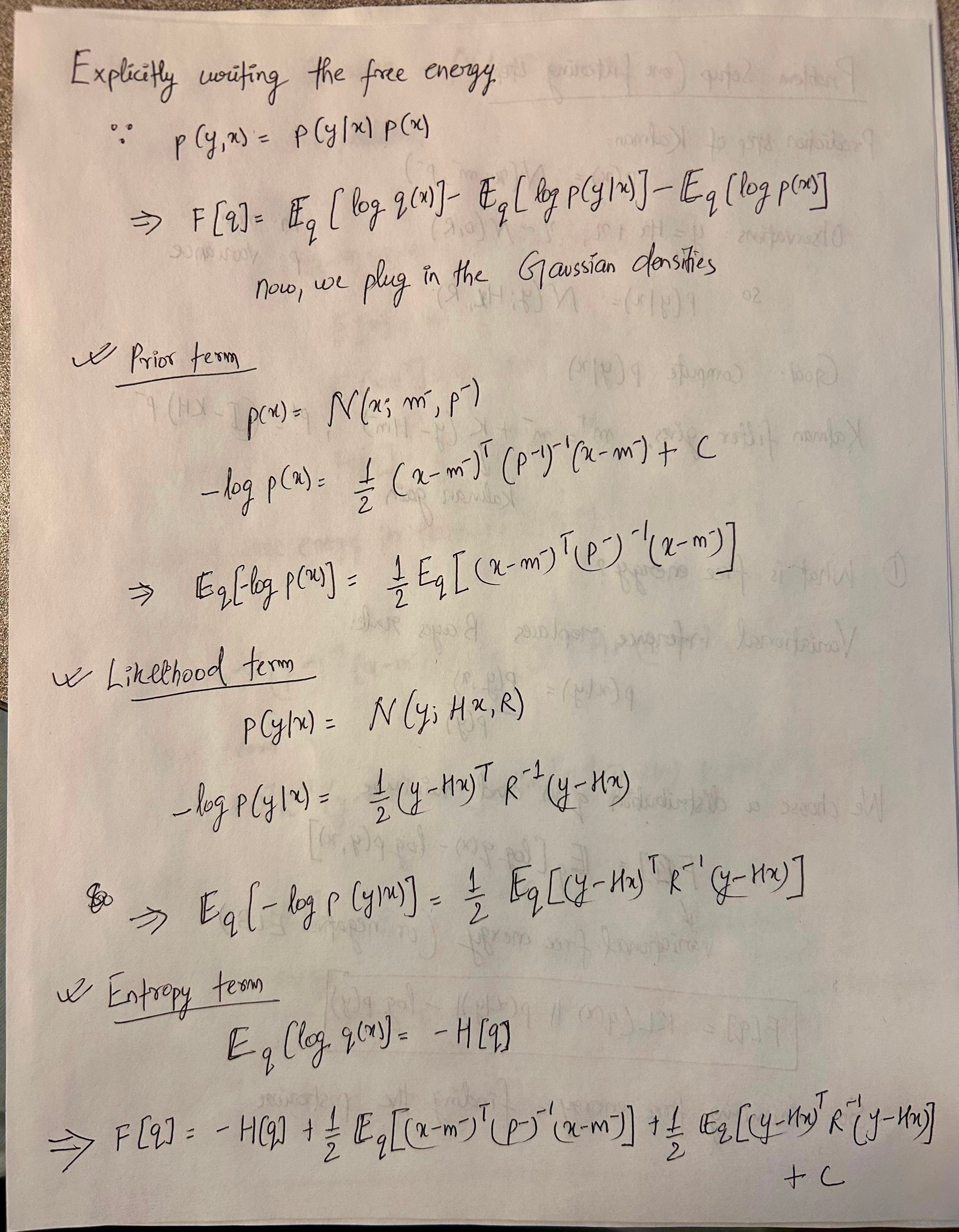
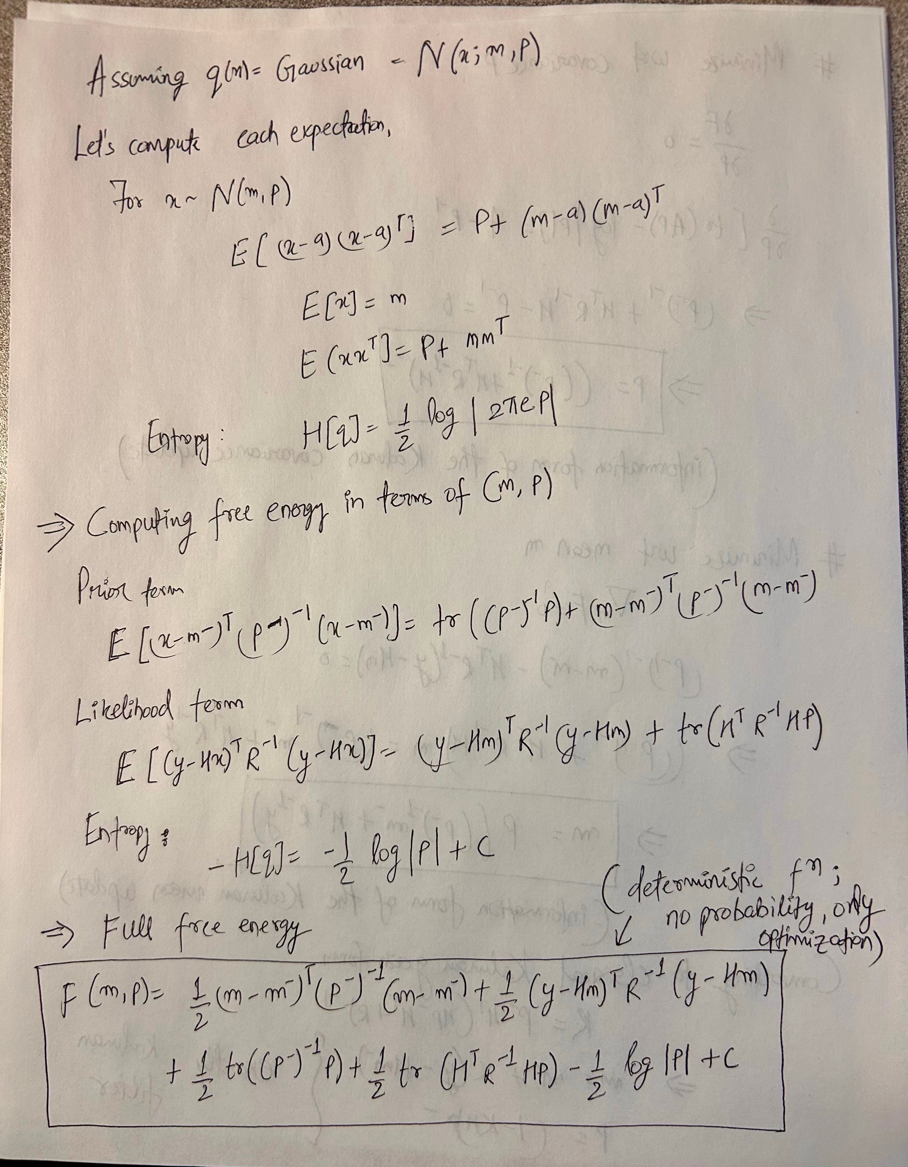
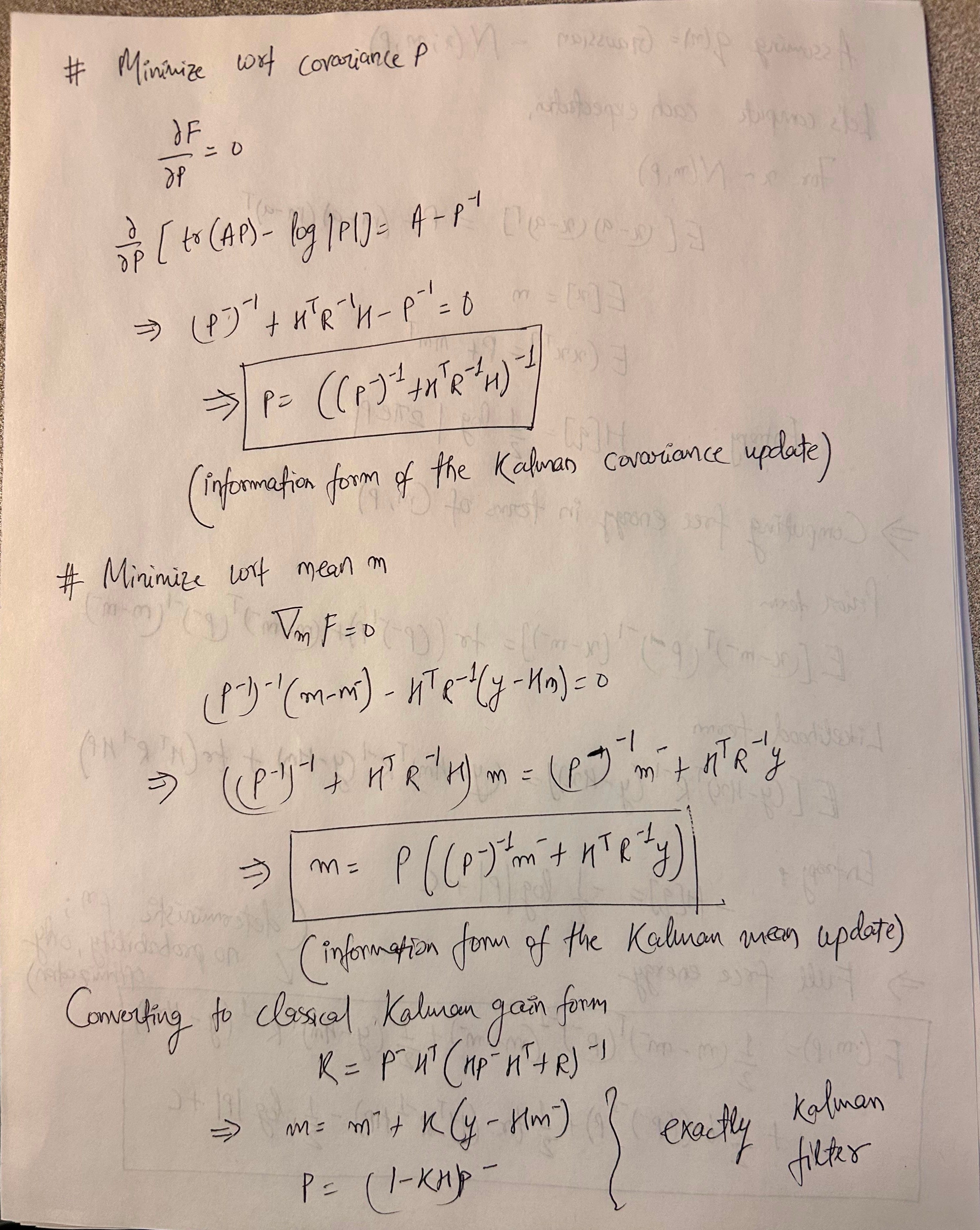
We’re gonna prove that free energy is actually a Kalman filter in linear-gaussian case. I am lazy, so here’s my handwritten derivations:

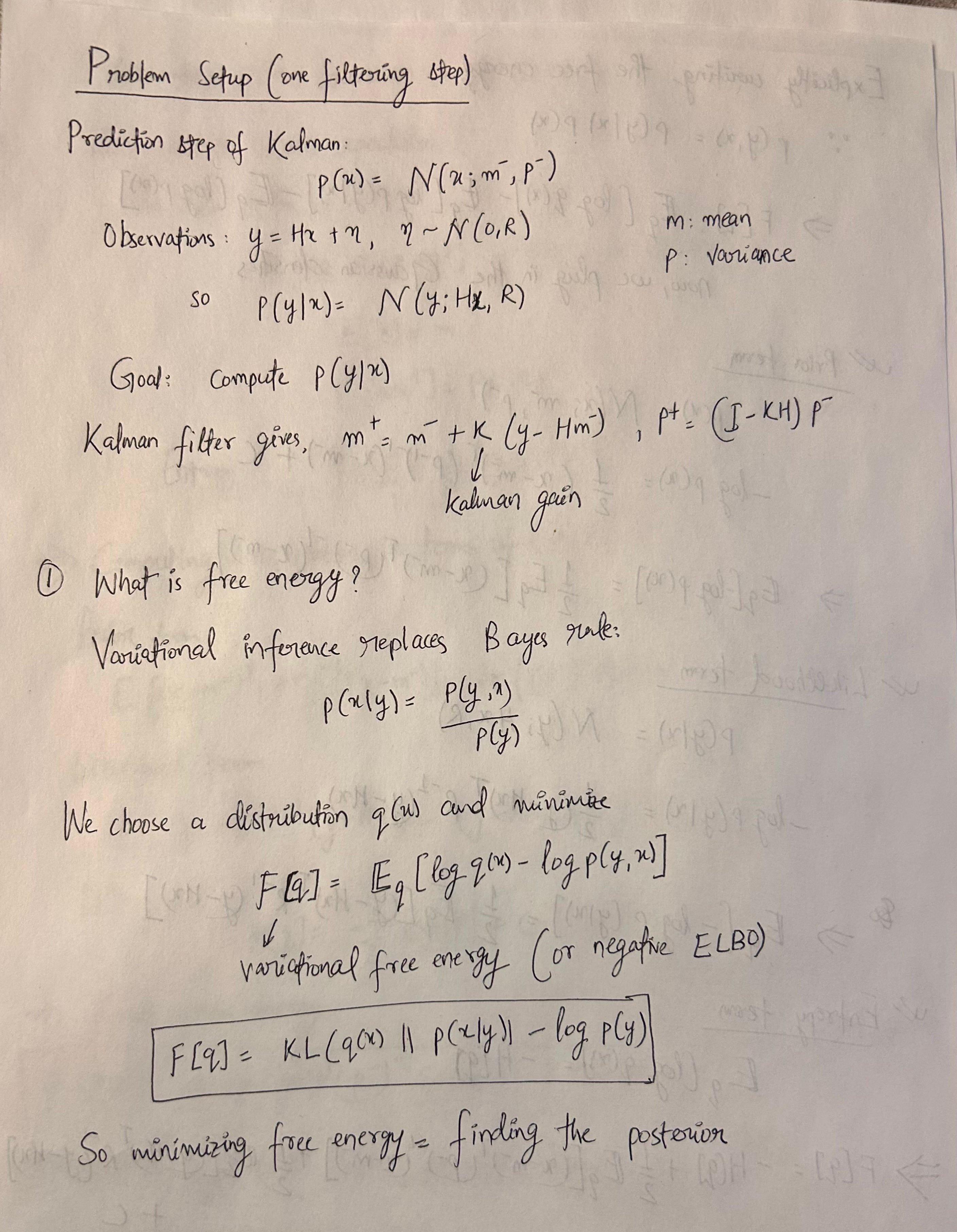
What just happened?

Filtering, which we previously treated as algebra:

\(p(x_t|o_{1:t})\)

is now a gradient flow minimizing free energy. Belief updates become error-correction dynamics.

In linear Gaussian systems, this reduces exactly to the Kalman filter. So predictive coding is not mystical neuroscience poetry. It’s filtering written as optimization.

Why does this reframing matter?

This perspective does something subtle but profound. It turns inference into dynamics. Instead of “Compute posterior using Bayes’ rule,” we now have: “Evolve internal state to minimize prediction error” — this shift is the bridge to neural world models.

Now we can connect this to RSSMs, Dreamer, and modern architectures.

Now we connect this to RSSMs, Dreamer, and modern architectures.

Modern neural world models:

• define the same generative structure

• train by minimizing ELBO

• use reconstruction + KL regularization

But they do not run iterative gradient descent per timestep.

They do something smarter.

They use amortized inference.

Instead of optimizing:

\(x_t = \arg \min F \)

They learn a function:

\(x_t = f_{\phi}(o_{\leq t})\)

The encoder replaces iterative free-energy minimization.

The neural network learns to approximate the fixed point of the gradient flow. This is the key bridge.

Predictive coding: iterative optimization over the latent state

Neural world models: learned inference network approximating that optimization

Both minimize free energy.

One does it explicitly.
One does it amortized.

Why reconstruction loss matters?

The predictive-coding view explains something people often misunderstand. Reconstruction loss is not cosmetic. It is the likelihood term in free energy.

If reconstruction loss is weak:

• prediction error disappears

• latents collapse

This connects directly to posterior collapse in VAEs and RSSMs.

The KL term:

• enforces temporal smoothness

• stabilizes latent dynamics

• prevents degenerate inference

All of this is visible directly in the free-energy formulation.

Surprise minimization is not control

Important clarification: Free-energy minimization explains perception.

It explains filtering. It does not automatically explain control.

Minimizing surprise passively:

• stabilizes internal representations

• explains sensory inference

Control requires:

• counterfactual rollouts

• action-conditioned transitions

• reward optimization

Later, we can talk about expected free energy and active inference. But for now:

Predictive coding = perception as error correction.

---

Summarizing the two views,

Classical filtering: posterior recursion, Bayes’ rule, algebraic update, closed-form in linear case

Predictive coding: gradient descent on free energy, error correction dynamics, local update rules, naturally implemented in neural systems.

Both solve the same problem — they are two coordinate systems over the same object.

A world model is not just a probability distribution. It is a dynamical system that resists surprise.

Filtering is not about computing posteriors. It’s about evolving the internal state to cancel prediction errors. Neural world models do the same thing; they just learn to do it in one forward pass.

~Ashutosh