
The real problem world models solve
We don't need a model, we need a state


Consider an agent interacting with an environment over discrete time steps t.
One crucial distinction here is that the agent never sees the ground-truth state. It only has the history of interactions:
The goal or the control objective is to find a policy that maximizes expected future returns. However, planning/control is challenging in historical contexts. The central move is to find a state (s_t) that compresses history while retaining all the information needed for prediction and control. Formally, the goal or objective can be defined as:
The ideal state is a sufficient statistic of history for the future:
This is the “world model” problem in its cleanest form:
such that the above sufficient statistic equation holds approximately.
Let’s break down the “problem” with targets
Target A: Predictive Modeling
Learn a model of future observables:
This is enough to do many things (imitating, forecasting), but not necessarily control, because rewards and goals may depend on latent factors that are weakly expressed in pixels.
Target B: Control-sufficient Modeling
Learn a state that is sufficient for value:
This is weaker than full prediction (we can ignore nuisance factors), but harder to ensure without either
explicit reward modeling or
coverage assumptions
A “world model” used for planning is usually trying to approximate Target A plus the parts of Target B needed for decision making.
Why end-to-end Model-free RL struggles here?
This is not “model-free never works”. It’s → There are structural failure modes that show up when we lack predictive structures (explanation in a bit).
A model-free agent (e.g., DQN, PPO) attempts to map the history of states, h_t → a_t directly (or h_t → V(h_t)). Why does it lead to structural failures?
High dimensionality: h_t grows linearly with time. Naively treating h_t as input is computationally intractable.
Sample Inefficiency: The agent must implicitly learn the physics of the world through the reward signal. If rewards are sparse, the agent receives no feedback on whether it understands the environment’s dynamics.
Lack of counterfactuals: A model-free agent answers, “What action is best?” It cannot answer “What would have happened if I did X?”
Now, what do we mean by “lacking predictive structures”?
Partial observability → aliasing → inconsistent value targets
If two latent states x and x’ produce the same observation o but require different optimal actions, then any policy is provably insufficient. We need memory/belief.
Model-free methods that train the policy (or shallow memory) can converge to brittle compromises because of these ambiguities.
Credit assignment through latent causes
Rewards often depend on unobserved factors (intent, friction, occluded agents). Without a predictive internal state, gradients push on spurious correlates in the observation space (“shortcut features”).
We get representations that are predictive of reward on the dataset, not of dynamics.
Compounding distribution shift under policy improvement
Even if we learn Q(o, a) well from data from the learned policy, policy improvement changes the distribution. In high-dimensional observation spaces, the support mismatch becomes severe, and model-free bootstrapping can amplify errors.
World models attack this by learning a structure shared across policies: transitions and observation generation.
Sample complexity: “learning dynamics implicitly” is expensive
A model-free agent can be viewed as trying to learn a function:
\((h_t, a_t) \rightarrow \text{action that implictly marginalizes over future trajectories}\)A world model factorizes the problem:
learn short-horizon predictive structure
Then plan/control using that structure
This factorization isn’t free (model bias), but it can dramatically reduce interaction needs when the factorizations match reality.
The World Model Hypothesis
To solve this efficiently, we hypothesize that the history (h_t) can be compressed into a compact Belief state (or latent state) z_t that captures all information necessary to predict the future. This is the Markov property applied to the latent space.
A World Model is explicitly learning the distributions T and O (and often R).
Mathematically, we decompose the problem into:
The first few lines of code
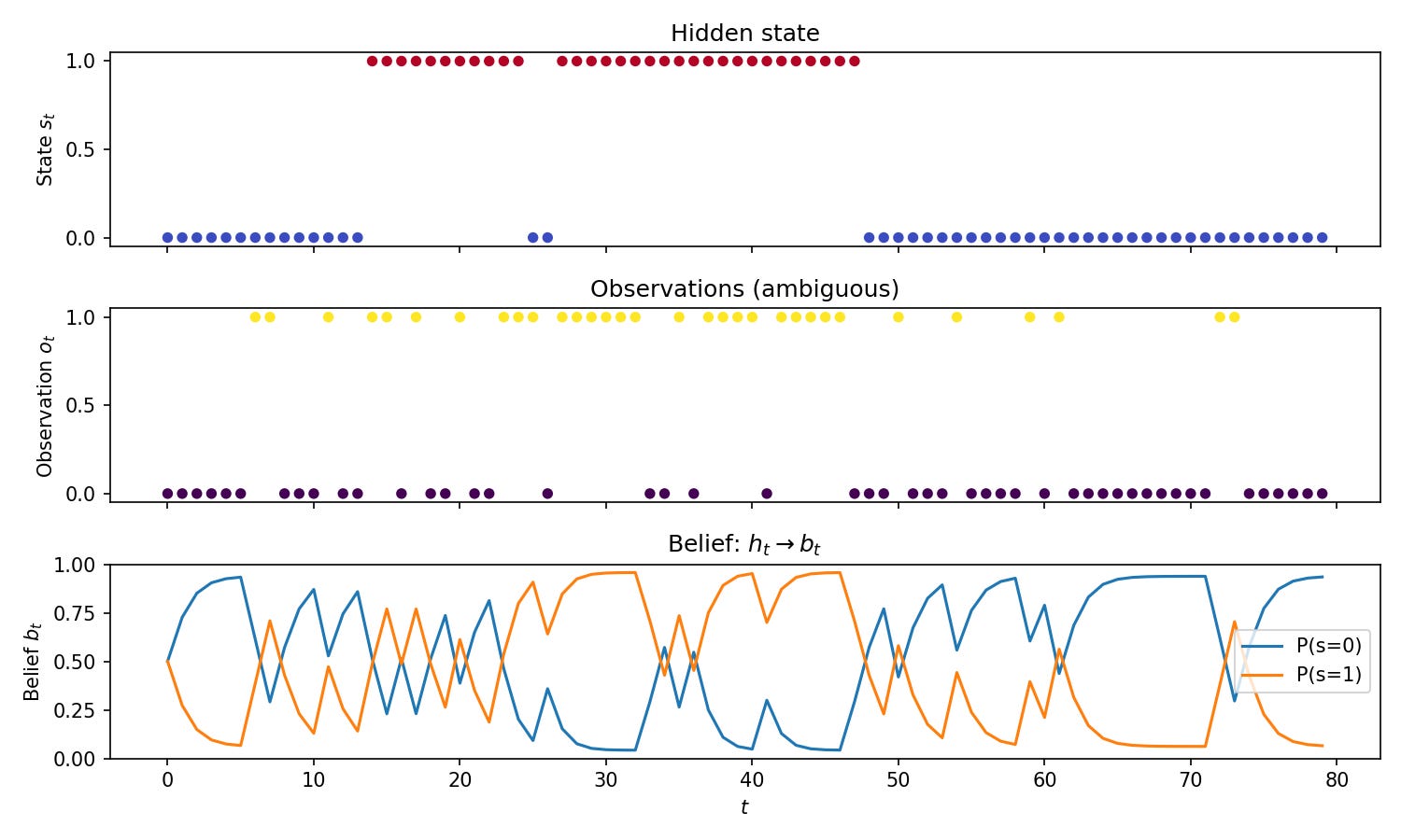
Here’s a minimal implementation of partial observability. A two-state Markov chain evolves in the background while we only see noisy observations. Because the emission model is ambiguous (both states can produce either observation with different probabilities), we cannot infer the true state from a single observation.
The code defines the transition and emission matrices, implements the belief update recursion (which we’ll derive in the next section), and generates a trajectory.
import numpy as np
import matplotlib.pyplot as plt

np.random.seed(42)

# 2-state POMDP: states 0,1; observations 0,1 (ambiguous)
P = np.array([[0.9, 0.1], [0.1, 0.9]])  # transition P(s'|s)
O = np.array([[0.8, 0.2], [0.3, 0.7]])  # emission P(o|s) — ambiguous


def step(s):
    s = np.random.choice(2, p=P[s])
    o = np.random.choice(2, p=O[s])
    return s, o

def belief_update(b, o):
    b = O[:, o] * (P.T @ b)
    return b / b.sum()

def generate(T=50):
    s = np.random.randint(2)
    b = np.array([0.5, 0.5])
    states, obs, beliefs = [s], [np.random.choice(2, p=O[s])], [b.copy()]
    for _ in range(T - 1):
        s, o = step(s)
        b = belief_update(b, o)
        states.append(s)
        obs.append(o)
        beliefs.append(b.copy())
    return np.array(states), np.array(obs), np.array(beliefs)
The plot shows the hidden state, the observations, and the belief over time, illustrating the idea that we need a belief state as a sufficient statistic rather than raw history.
What’s next?
We will derive how the belief updates using recursion and derive the Kalman filter from scratch. We’re gonna show prediction vs correction as two distinct operations, and explain covariance as “uncertainty budget” — filtering is the original world model (Kalman as Bayes).
~Ashutosh